


Informatics Educational Institutions & Programs


The Newton fractal is a boundary set in the complex plane which is characterized by Newton's method applied to a fixed polynomial p(z) ∈ [z] or transcendental function. It is the Julia set of the meromorphic function z ↦ z − p(z)/p′(z) which is given by Newton's method. When there are no attractive cycles (of order greater than 1), it divides the complex plane into regions Gk, each of which is associated with a root ζk of the polynomial, k = 1, …, deg(p). In this way the Newton fractal is similar to the Mandelbrot set, and like other fractals it exhibits an intricate appearance arising from a simple description. It is relevant to numerical analysis because it shows that (outside the region of quadratic convergence) the Newton method can be very sensitive to its choice of start point.

Almost all points of the complex plane are associated with one of the deg(p) roots of a given polynomial in the following way: the point is used as starting value z0 for Newton's iteration zn + 1 := zn − p(zn)/p'(zn), yielding a sequence of points z1, z2, …, If the sequence converges to the root ζk, then z0 was an element of the region Gk. However, for every polynomial of degree at least 2 there are points for which the Newton iteration does not converge to any root: examples are the boundaries of the basins of attraction of the various roots. There are even polynomials for which open sets of starting points fail to converge to any root: a simple example is z3 − 2z + 2, where some points are attracted by the cycle 0, 1, 0, 1… rather than by a root.
An open set for which the iterations converge towards a given root or cycle (that is not a fixed point), is a Fatou set for the iteration. The complementary set to the union of all these, is the Julia set. The Fatou sets have common boundary, namely the Julia set. Therefore, each point of the Julia set is a point of accumulation for each of the Fatou sets. It is this property that causes the fractal structure of the Julia set (when the degree of the polynomial is larger than 2).
To plot images of the fractal, one may first choose a specified number d of complex points (ζ1, …, ζd) and compute the coefficients (p1, …, pd) of the polynomial
- .

Then for a rectangular lattice

of points in , one finds the index k(m,n) of the corresponding root ζk(m,n) and uses this to fill an M × N raster grid by assigning to each point (m,n) a color fk(m,n). Additionally or alternatively the colors may be dependent on the distance D(m,n), which is defined to be the first value D such that |zD − ζk(m,n)| < ε for some previously fixed small ε > 0.
Generalization of Newton fractals
A generalization of Newton's iteration is

where a is any complex number.[1] The special choice a = 1 corresponds to the Newton fractal. The fixed points of this map are stable when a lies inside the disk of radius 1 centered at 1. When a is outside this disk, the fixed points are locally unstable, however the map still exhibits a fractal structure in the sense of Julia set. If p is a polynomial of degree d, then the sequence zn is bounded provided that a is inside a disk of radius d centered at d.
More generally, Newton's fractal is a special case of a Julia set.
-
 Newton fractal for three degree-3 roots p(z) = z3 − 1, coloured by number of iterations required
 -
 Newton fractal for three degree-3 roots p(z) = z3 − 1, coloured by root reached
 -
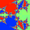
 Newton fractal for p(z) = z3 − 2z + 2. Points in the red basins do not reach a root.
 -
 Newton fractal for a 7th order polynomial, colored by root reached and shaded by rate of convergence.
 -
 Newton fractal for p(z) = z8 + 15z4 − 16
 -
 Newton fractal for p(z) = z5 − 3iz3 − (5 + 2i)z2 + 3z + 1, coloured by root reached, shaded by number of iterations required.
 -
 Newton fractal for p(z) = sin z, coloured by root reached, shaded by number of iterations required
 -
 Another Newton fractal for p(z) = sin z
 -
 Generalized Newton fractal for p(z) = z3 − 1, a = −1/2. The colour was chosen based on the argument after 40 iterations.
 -
 Generalized Newton fractal for p(z) = z2 − 1, a = 1 + i.
 -
 Generalized Newton fractal for p(z) = z3 − 1, a = 2.
 -
 Generalized Newton fractal for p(z) = z4 + 3i − 1, a = 2.1.
 -
 p(z) = z6 + z3 - 1
 -
 p(z) = sin z - 1
 -
 p(z) = sin z - 1
 -
 p(z) = cosh z - 1
 -
 p(z) = cosh z - 1
 -
 p(z) = z20 - 2z + 2


Serie : p(z) = zn- 1
-
 p(z) = z3 - 1, a=1
 -
 p(z) = z3 - 1, a=2
 -
 p(z) = z4 - 1, a=1
 -
 p(z) = z4 - 1, a=2
 -
 p(z) = z5 - 1, a=1
 -
 p(z) = z5 - 1, a=2
 -
 p(z) = z6 - 1, a=1
 -
 p(z) = z7 - 1, a=1
 -
 p(z) = z8 - 1, a=1
 -
 p(z) = z10 - 1, a=1


Other fractals where potential and trigonometric functions are multiplied. p(z) = zn*Sin(z) - 1
-
 p(z) = z2*Sin(Z) - 1, a=1
 -
 p(z) = z2*Sin(Z) - 1, a=1 (zoom)
 -
 p(z) = z3*Sin(Z) - 1, a=1
 -
 p(z) = z4*Sin(Z) - 1, a=1
 -
 p(z) = z4*Sin(Z) - 1, a=1 (zoom)
 -
 p(z) = z5*Sin(Z) - 1, a=1
 -
 p(z) = z6*Sin(Z) - 1, a=1
 -
 p(z) = z6*Sin(Z) - 1, a=1 (zoom)


Nova fractal
The Nova fractal invented in the mid 1990s by Paul Derbyshire,[2][3] is a generalization of the Newton fractal with the addition of a value c at each step:[4]

The "Julia" variant of the Nova fractal keeps c constant over the image and initializes z0 to the pixel coordinates. The "Mandelbrot" variant of the Nova fractal initializes c to the pixel coordinates and sets z0 to a critical point, where[5]

Commonly-used polynomials like p(z) = z3 − 1 or p(z) = (z − 1)3 lead to a critical point at z = 1.
-
 Animated "Julia" Nova fractal for p(z) = z3 − 1 with c going from −1 to 1, colored by root reached.
 -
 Animated "Julia" Nova fractal for p(z) = z3 − 1 with c = 1/2eiφ and φ going from 0 to 2π, colored by root reached.


Implementation
In order to implement the Newton fractal, it is necessary to have a starting function as well as its derivative function:

The three roots of the function are

The above-defined functions can be translated in pseudocode as follows:
//z^3-1
float2 Function (float2 z)
{
	return cpow(z, 3) - float2(1, 0); //cpow is an exponential function for complex numbers
}

//3*z^2
float2 Derivative (float2 z)
{
	return 3 * cmul(z, z); //cmul is a function that handles multiplication of complex numbers
}
It is now just a matter of implementing the Newton method using the given functions.
float2 roots[3] = //Roots (solutions) of the polynomial
{
	float2(1, 0),
	float2(-.5, sqrt(3)/2),
	float2(-.5, -sqrt(3)/2)
};

color colors[3] =  //Assign a color for each root
{
    red,
    green,
    blue
}

For each pixel (x, y) on the target, do:
{
	zx = scaled x coordinate of pixel (scaled to lie in the Mandelbrot X scale (-2.5, 1))
    zy = scaled y coordinate of pixel (scaled to lie in the Mandelbrot Y scale (-2, 1))

    float2 z = float2(zx, zy); //z is originally set to the pixel coordinates

	for (int iteration = 0;
	     iteration < maxIteration;
	     iteration++;)
	{
		z -= cdiv(Function(z), Derivative(z)); //cdiv is a function for dividing complex numbers

        float tolerance = 0.000001;

		for (int i = 0; i < roots.Length; i++)
		{
		    float2 difference = z - roots[i];

			//If the current iteration is close enough to a root, color the pixel.
			if (abs(difference.x) < tolerance && abs (difference.y) < tolerance)
			{
				return colors[i]; //Return the color corresponding to the root
			}
		}

    }

    return black; //If no solution is found
}
See also
References
- ^ Simon Tatham. "Fractals derived from Newton–Raphson".
- ^ Damien M. Jones. "class Standard_NovaMandel (Ultra Fractal formula reference)".
- ^ Damien M. Jones. "dmj's nova fractals 1995-6".
- ^ Michael Condron. "Relaxed Newton's Method and the Nova Fractal".
- ^ Frederik Slijkerman. "Ultra Fractal Manual: Nova (Julia, Mandelbrot)".
Further reading
- J. H. Hubbard, D. Schleicher, S. Sutherland: How to Find All Roots of Complex Polynomials by Newton's Method, Inventiones Mathematicae vol. 146 (2001) – with a discussion of the global structure of Newton fractals
- On the Number of Iterations for Newton's Method by Dierk Schleicher July 21, 2000
- Newton's Method as a Dynamical System by Johannes Rueckert
- Newton's Fractal (which Newton knew nothing about) by 3Blue1Brown, along with an interactive demonstration of the fractal on his website, and the source code for the demonstration
